Friday, March 29, 2013

Bitmap Index Overview


Bitmap Index

Overview 

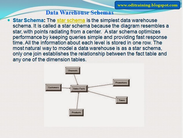
A bitmap index is an indexing method that can provide both performance benefits and storage savings. Bitmap indexes are particularly useful for data warehousing environments because data is usually updated less frequently and ad hoc queries are more common.
While B-tree indexes are the most effective method for “high-cardinality” data (data where there are many possible values, such as customer_name or phone_number), bit-mapped indexes are best for “low-cardinality” data (such as a column to indicate a person’s gender, which contains only two possible values: MALE and FEMALE).

Building a bitmap index

A portion of a sample company’s customer data is shown below:
customer#     marital_status     region     gender     income_level
101           single             east       male       bracket_1
102           married            central    female     bracket_4
103           married            west       female     bracket_2
104           divorced           west       male       bracket_4
105           single             central    female     bracket_2
106           married            central    female     bracket_3
Since MARITAL_STATUS, REGION, GENDER, and INCOME_LEVEL are all “low-cardinality” columns (there are only three possible marital status’s, three possible regions, two possible genders, and four possible income levels), it’s appropriate to create bitmap indexes on these columns. A bitmap index should not be created on CUSTOMER#, because this is a “high-cardinality” column, in fact it is the primary key of this table which means each value is unique. Instead, an ordinary, unique B-tree index should be created on this column in order to provide the most efficient representation and retrieval.
The bitmap index for the REGION column consists of three separate bit-maps, one for each region. These bit-maps are shown below:
region='east'   region='central'   region='west'
      1               0                  0
      0               1                  0
      0               0                  1
      0               0                  1
      0               1                  0
      0               1                  0
Each entry (or “bit”) in the bitmap corresponds to a single row of the CUSTOMER table. The value of each bit depends upon the values of the corresponding row in the table. For example, the bitmap REGION=‘east’ contains a one as its first bit; this is due to the fact that the REGION is ‘east’ in the first row of the CUSTOMER table. The bitmap REGION=‘east’ has a zero for its other bits because none of the other rows of the CUSTOMER table contain ‘east’ as their value for REGION. With this scheme, it is impossible for a single row to have a bit set in more than one bitmap for that column.

Using a bitmap index

Suppose you want to look at the demographic trends of the company’s customers. A sample question might be: “How many of our married customers live in the central or west regions?” which could be coded in an SQL query as:
select count(*) from customer 
 where marital_status = 'married' 
   and region in ('central','west');
Bitmap indexes can be used to process this query. One bitmap is used to evaluate each predicate, and the bitmaps are logically combined to evaluate the AND’s and the OR’s. For example:

By counting the number of 1’s in the resulting bitmap above, the result of this query can be easily computed. If you further wanted to know the specific customers that satisfied the criteria, instead of simply the number of customers, the resulting bitmap would be used to access the table. In this manner, bitmap indexes are said to cooperate with each other. The bitmap indexes for multiple columns can be AND’ed or OR’ed together to determine the one bitmap that will satisfy the query. All of this is done before the table is even accessed. B-tree indexes do not cooperate with each other. Multiple bitmap indexes can be used to satisfy this query. Only one B-tree index can be used for this query, even if multiple B-tree indexes exist. 

When to use a bitmap index

There are three things to consider when choosing an index method: 
  • performance
  • storage
  • maintainability
The advantage for using bitmap indexes are their performance impact for certain queries and their relatively small storage requirements. Note however that bitmap indexes are not applicable to every query and bitmap indexes, like B-tree indexes, can impact the performance of insert, update, and delete statements. When you modify table that has a bitmap index, the table must be locked to update the bitmaps. This can lead to poor performance in situations where the table has a high degree of modification concurrency. 

Performance Considerations

Bitmap indexes can provide very impressive performance improvements. Execution times of certain queries may improve by several orders of magnitude. The queries that benefit the most from bitmap indexes have the following characteristics:
  • the WHERE-clause contains multiple predicates on low-cardinality columns
  • the individual predicates on these low-cardinality columns select a large number of rows
  • bitmap indexes have been created on some or all of these low-cardinality columns
  • the tables being queried contain many rows
An advantage of bitmap indexes is that multiple bitmap indexes can be used to evaluate the conditions on a single table. Thus, bitmap indexes are very useful for complex ad hoc queries that contain lengthy WHERE-clauses.

Storage considerations

Bitmap indexes incur a small storage cost and have a significant storage savings over B-tree indexes. A bitmap index can require 100 times less space than a B-tree index for a low-cardinality column.
Important Note: 
A strict comparison of the relative sizes of B-tree and bitmap indexes is not an accurate measure for selecting bitmap over B-tree indexes. Because of the performance characteristics of bitmap indexes and B-tree indexes, you should continue to maintain B-tree indexes on your high-cardinality data. Bitmap indexes should be considered primarily for your low-cardinality data.
With bitmap indexes, the problems associated with multiple-column B-tree indexes is solved because bitmap indexes can be efficiently combined during query execution; they cooperate with each other. Note that while the bitmap indexes may not be quite as efficient during execution as the appropriate concatenated B-tree indexes, the space savings provided by bitmap indexes can often more than justify their utilization.
The net storage savings will depend upon a database’s current usage of B-tree indexes:
  • A database that relies on single-column B-tree indexes on high-cardinality columns will not observe significant space savings (but should see significant performance increases). 
     
  • A database containing a significant number of concatenated B-tree indexes could reduce its index storage usage by 50% or more, while maintaining similar performance characteristics.
     
  • A database that lacks concatenated B-tree indexes because of storage constraints will be able to use bitmap indexes and increase performance with minimal storage costs.
Bitmap indexes are best for read-only or light OLTP environments. Because there is no effective method for locking a single bit, row-level locking is not available for bitmap indexes. Instead, locking for bitmap indexes is effectively at the block level which can impact heavy OLTP environments. Note also that like other types of indexes, updating bitmap indexes is a costly operation.
Though bitmap indexes are not appropriate for databases with a heavy load of insert, update, and delete operations, their effectiveness in a data warehousing environment is not diminished. In such environments, data is usually maintained via bulk inserts and updates. For these bulk operations, rebuilding or refreshing bitmap indexes is an efficient operation. The storage savings and performance gains provided by bitmap indexes can provide tremendous benefits to data warehouse users.

Performance/storage characteristics

In preliminary testing of bitmap indexes, certain queries ran up to 100 times faster. The bitmap indexes on low cardinality columns were also about ten times smaller than B-tree indexes on the same columns. In these tests, the queries containing multiple predicates on low-cardinality data experienced the most significant speedups. Queries that did not conform to this characteristic were not assisted by bitmap indexes.

Example CREATE Syntax

CREATE BITMAP INDEX myindex ON mytable(col1);

Example scenarios

The following sample queries on the CUSTOMERS table demonstrate the variety of query-processing techniques that are necessary for optimal performance.
  Example #1:   Single predicate on a low-cardinality attribute.
select * from customers 
 where gender = 'male';
Best approach: parallel table scan
This query will return approximately 50% of the data. Since we will be accessing such a large number of rows, it is more efficient to scan the entire table rather than use either bitmap indexes or B-tree indexes. To minimize elapsed time, the Server should execute this scan in parallel.
  Example #2:   Single predicate on a high-cardinality attribute.
select * from customers 
 where customer# = 101;
Best approach: conventional unique index
This query will retrieve at most one record from the employee table. A B-tree index or hash cluster index is always appropriate for retrieving a small number of records based upon criteria on the indexed columns.
  Example #3:   Multiple predicates on low-cardinality attributes
select * from customers 
 where gender = 'male' 
   and region in ('central','west') 
   and marital_status in ('married', 'divorced');
Best approach: bit-mapped index
Though each individual predicate specifies a large number of rows, the combination of all three predicates will return a relatively small number of rows. In this scenario, bitmap indexes provide substantial performance benefits.
  Example #4:   Multiple predicates on both high-cardinality and low-cardinality attributes.
select * from customers 
 where gender = 'male' 
   and customer# < 100;
Best approach: B-tree index on CUSTOMER#
This query returns a small number of rows because of the highly selective predicate on CUSTOMER#. It is more efficient to use a B-tree index on CUSTOMER# than to use a bitmap index on GENDER.
In each of the previous examples, the Oracle cost-based optimizer transparently determines the most efficient query-processing technique.

A special note on cardinality

As has been noted, bitmap indexes work best with low cardinality. The most often examples of columns with low cardinality are gender columns (Male/Female) and truth columns (True/False). In some situtations, these columns should not even be candidates for any index, let alone bitmap indexes. If you have a company database and there is a table named EMPLOYEES, then you might have a column called GENDER. If your company is representative of the general population distribution, then approximately have of your company will be male and the other half will be female. If your query is looking for all of the female employees in your table, then approximately half of the rows of data in that table would be returned. When you return that many rows from a table, a full table scan would be faster than using any index. So while bitmap indexes should be used for low cardinality columns, there is a danger in columns that have too low of a cardinality.
That being said, bitmap indexes, even on such low cardinality columns, can still help with queries. As has been shown above, bitmap indexes can cooperate with each other. When you issue a query such as the follows:
select * from customers 
 where gender = 'male' 
   and region in ('central','west');
This query can use the bitmap index on the GENDER column to filter out approximately half of the rows. The bitmap index on the REGION column can be used to further filter the rows down. In cooperating together, bitmap indexes achieve their greatest benefits.

Bitmap Join Indexes


Bitmap Join Indexes

Bitmap indexes were introduced back in Oracle 8. Now with Oracle 9i, we can create bitmap join indexes. Bitmap join indexes represent the join of columns in two or more tables. With a bitmap join index, the value of a column in one table (generally a dimension table) is stored with the associated ROWIDs of the like value in the other tables that the index is defined on. This provides fast join access between the tables-if that query uses the columns of the bitmap join index.  In a data-warehouse environment, a bitmap join index might be a more efficient way of accessing data than a materialized view join. When using a bitmap join index in a warehouse or EIS environment, you would create the join using an equi-inner join between the primary key column(s) of the dimension tables and the foreign key column(s) of the fact table.
You create a bitmap join index using the CREATE BITMAP INDEX command. Here is an example of the creation of a bitmap index:
CREATE BITMAP INDEX my_bitmap_index
ON fact_table(dimension_table.col_2)
FROM dimension_table, fact_table
WHERE dimension_table.col1=fact_table.col1;
There are a few restrictions on bitmap join indexes that you should be aware of. These include the following:
  • The bitmap join index is built on a single table. In the previous example, the bitmap join index is built on the FACT_TABLE table.
     
  • Oracle will allow only one of the tables of a bitmap join index to be updated, inserted, or deleted from at a time.
     
  • You cannot join the same table to itself, that is, no table can appear twice in the FROM clause.
     
  • A bitmap join index cannot be created on an index-organized table or a temporary table.
     
  • Every column in the bitmap join index must be present in one of the associated dimension tables. The joins in the bitmap index must form either a star or snowflake schema.
     
  • Either primary key columns or unique constraints must be created on the columns that will be join columns in the bitmap join index.
     
  • All the primary key columns of the dimension table must be part of the join criteria of the bitmap join index.
     
  • All restrictions on normal bitmap indexes apply to bitmap join indexes.
     
  • You cannot create a bitmap join index on an IOT.
This query can use the bitmap index on the GENDER column to filter out approximately half of the rows. The bitmap index on the REGION column can be used to further filter the rows down. In cooperating together, bitmap indexes achieve their greatest benefits.

SCD Type 2 error: ODI-1228:ORA-01747: invalid user.table.column, table.column, or column specification

ODI-1228: Caused By: java.sql.SQLSyntaxErrorException: ORA-01747: invalid user.table.column, table.column, or column specification


This is common issue.

While enabling your SCD table column SCD properties if you not enable "Overwrite On Change" 
this property simply

Goto =>SCD IKM=>select Ignore error option on Update Existing Rows.

Oracle Job Schedulers examples

Oracle Job Schedulers examples

The following code examples rely on the previously defined programs and schedules to show how the overloads of the create_job procedure are used.
BEGIN
  -- Job defined entirely by the CREATE JOB procedure.
  DBMS_SCHEDULER.create_job (
    job_name        => 'test_full_job_definition',
    job_type        => 'PLSQL_BLOCK',
    job_action      => 'BEGIN my_job_proc(''CREATE_PROGRAM (BLOCK)''); END;',
    start_date      => SYSTIMESTAMP,
    repeat_interval => 'freq=hourly; byminute=0',
    end_date        => NULL,
    enabled         => TRUE,
    comments        => 'Job defined entirely by the CREATE JOB procedure.');
END;
/
BEGIN
  -- Job defined by an existing program and schedule.
  DBMS_SCHEDULER.create_job (
    job_name      => 'test_prog_sched_job_definition',
    program_name  => 'test_plsql_block_prog',
    schedule_name => 'test_hourly_schedule',
    enabled       => TRUE,
    comments      => 'Job defined by an existing program and schedule.');
END;
/

Get a list of MViews depending on table using DBMS_MVIEW.GET_MV_DEPENDENCIES

DECLARE
   v_output   VARCHAR2 (2000);
   v_owner    VARCHAR2 (30);
   v_table    VARCHAR2 (30);
BEGIN
   v_owner := UPPER ('&&ENTER_OWNER_NAME');
   v_table := UPPER ('&&ENTER_TABLE_NAME');
   DBMS_MVIEW.GET_MV_DEPENDENCIES (v_owner || '.' || v_table, v_output);
   DBMS_OUTPUT.put_line (CHR (13));
   DBMS_OUTPUT.put_line
      ('Materialized Views Dependent on table      &&ENTER_OWNER_NAME..&&ENTER_TABLE_NAME'
      );
   DBMS_OUTPUT.put_line (CHR (13));
   DBMS_OUTPUT.put_line (v_output);
END;
/

Thursday, March 28, 2013

B-Tree Index


B-Tree  Index

A B-tree is a special data structure format for an index that allows rapid access of the data in the index. One of the properties of this data structure is that the index is always balanced. That means that each node at the lowest level is equidistant from the top most node, or the root node of the tree. And each side of the index has the same number of nodes. The nodes at the lowest levels are known as leaf nodes. All other nodes are known as branch nodes. Branches point to other branches or leaf nodes. Leaf nodes store value-rowid pairs, or the values of the indexed columns and the rowid that points to a distinct row that has those values.  The actual distribution will depend on the number of data values in each range of values in a B-tree with the overall goal to reduce the number of required levels that must be traversed to get to a specific value. The advantages of a B-tree structure are:
  • All leaf blocks are of the same depth (number of values).
     
  • The height of the B-tree, or the total number of nodes from the root to any leaf, is typically pretty small. In some cases, the root node is the only leaf node and the height is 1. As the table gets more rows inserted into it, the index must grow to accommodate this. But even in tables with over 1 million rows, the B-tree index typically has a height of 3. In the very largest of tables, the height may only be 4. This means that for even the largest of tables, it only takes 4 blocks to find the rowid of the row you are looking for. This is extremely efficient.
     
  • In the case of randomly entered data, the B-tree stays balanced automatically. In fact, the B-tree stays balanced no matter what data is entered into it.
     
  • All blocks of a B-tree index are three-quarters full (on the average), allowing insertion without rebuild.
     
  • B-trees provide excellent performance for all types of selects.
     
  • Insert, update, and deletes tend to be efficient in a B-tree structure.
     
  • B-tree performance stays optimal even when tables vary from small to large.
  • OLAP databases we will B-tree indexes

World of ETL Tools Available ... sooooooomany etl tools.....

I found the below list available ETL tools on google. sooooooomany etl tools.....
World of ETL Tools Available
ETL Product Name
Vendor
ActaWorks
Acta Technologies
Amadea
ISoft
ASG-XPATH
Allen Systems Group
AT Sigma W-Import
Advanced Technologies
AutoImport
White Crane Systems
Automatic Data Warehouse Builder
Gilbert Babin
Blue Data Miner
Blue Data
Catalyst
Synectics Solutions
CDB/Superload
CDB Software
Cerebellum Portal Integrator
Cerebellum Software
Checkmate
BitbyBit International Ltd.
Chyfo
Ispirer Systems
CMS TextMap
Cornerstone Management Systems
Compleo
Symtrax
Content Connect
One Page
Convert /IDMS-DB, Convert/VSAM
Forecross Corporation
Conversions Plus
DataViz
Copy Manager
Information Builders, Inc.
CoSORT
Innovative Routines International, Inc.
CrossXpress
Cross Access Corporation
Cubeware Importer
CubeWare
Cyklop
Tokab Software AB
Data Cycle
APE Software Components S.L.
Data Exchange
XSB
Data EXTRactor
DogHouse Enterprises
Data Flow Manager
Peter's Software
Data Junction, Content Extractor
Data Junction
Data Manager
Joe Spanicek
Data Mapper
Applied Database Technology
Data Migration Tools
Friedman & Associates
Data Migrator for SAP, PeopleSoft
Information Builders, Inc.
Data Propagation System
Treehouse Software
Data Warehouse Tools
Javacorporate
Data3
Inform Information Systems
DataBlaster 2
Bus-Tech, Inc.
DataBrix Data Manager
Lakeview Technology
DataConvert
Metadata Information Partners
DataDigger
Donnell Systems
DataExchanger SRV
CrossDataBase Technology
Datagration
Paladyne
DataImport
Spalding Software
DataLoad
Software Technologies Corporation
DataManager
Joe Spanicek
DataMIG
Dulcian, Inc.
DataMiner
Placer Group
DataMirror Constellar Hub
DataMirror Corporation
DataMirror Transformation Server
DataMirror Corporation
DataProF
IT Consultancy Group BV
DataPropagator
IBM
DataProvider
Order Software Company
DataPump for SAP R/3
Transcope AG
DataStage XE
Ascential Software
DataSuite
Pathlight Data Systems
Datawhere
Miab Systems Ltd.
DataX
Data Migrators
DataXPress
EPIQ Systems
DB/Access
Datastructure
DBMS/Copy
Conceptual Software, Inc.
DBridge
Software Conversion House
DEAP I
DEAP Systems
DecisionBase
Computer Associates
DecisionStream
Cognos
DECISIVE Advantage
InfoSAGE, Inc.
Departmental Suite 2000
Analytical Tools Inc.
DETAIL
Striva Technology
Distribution Agent for MVS
Sybase
DocuAnalyzer
Mobius Management
DQtransform
Metagon Technologies
DT/Studio
Embarcadero Technologies
DTS
Microsoft
e-Sense Gather
Vigil Technologies
e-zMigrate
e-zdata.net
eIntegration Suite
Taviz Technology
Environment Manager
WhiteLight Technology
ETI Extract
Evolutionary Technologies, Inc.
ETL Engine
FireSprout
ETL Manager
iWay Software
eWorker Portal, eWorker Legacy
entrinsic.com
EZ-Pickin's
ExcelSystems
FastCopy
SoftLink
File-AID/Express
CompuWare
FileSpeed
Computer Network Technology
Formware
Captiva Software
FOXTROT
EnableSoft, Inc.
Fusion FTMS
Proginet
Gate/1
Selesta
Génio
Hummingbird Communications Ltd.
Gladstone Conversion Package
Gladstone Computer Services
GoHunter
Gordian Data
Graphical Performance Series
Vanguard Solutions
Harvester
Object Technology UK
HIREL
SWS Software Services
iManageData
BioComp Systems
iMergence
iMergence Technologies
InfluX
Network Software Associates, Inc.
InfoLink/400
Batcom
InfoManager
InfoManager Oy
InfoRefiner, InfoTransport, InfoHub, InfoPump
Computer Associates
Information Discovery Platform
Cymfony
Information Logistics Network
D2K
InformEnt
Fiserv
InfoScanner
WisoSoftCom
InScribe
Critical Path
InTouch/2000
Blue Isle Software, Inc.
ISIE
Artaud, Courthéoux & Associés
John Henry
Acme Software
KM.Studio
Knowmadic
LiveTransfer
Intellicorp
LOADPLUS
BMC Software
Mainframe Data Engine
Flatiron Solutions
Manheim
PowerShift
Mercator
TSI International
Meta Integration Works
Meta Integration Technologies
MetaSuite
Minerva Softcare
MetaTrans
Metagenix
MineWorks/400
Computer Professional Systems
MinePoint
MinePoint
MITS
Management Information Tools
Monarch
Datawatch Corporation
Mozart
Magma Solutions
mpower
Ab Initio
MRE
SolutionsIQ
NatQuery
NatWorks, Inc
netConvert
The Workstation Group, Ltd.
NGS-IQ
New Generation Software
NSX Data Stager
NSX Software
ODBCFace
System Tech Consulting
OLAP Data Migrator
Legacy to Web Solutions
OmniReplicator
Lakeview Technology
OpalisRendezVous
Opalis
Open Exchange
IST
OpenMigrator
PrismTech
OpenWizard Professional
OpenData Systems
OptiLoad
Leveraged Solutions, Inc.
Oracle Warehouse Builder
Oracle Corporation
Orchestrate
Torrent Systems Inc.
Outbound
Firesign Computer Company
Parse-O-Matic
Pinnacle Software
ParseRat
Guy Software
pcMainframe
cfSOFTWARE
PinnPoint Plus
Pinnacle Decision Systems
PL/Loader
Hanlon Consulting
PointOut
mSE GmbH
Power*Loader Suite
SQL Power Group
PowerDesigner WarehouseArchitect
Powersoft
PowerMart
Informatica
PowerStage
Sybase
Rapid Data
Open Universal Software
Relational DataBridge
Liant Software Corporation
Relational Tools
Princeton Softech
ReTarGet
Tominy
Rodin
Coglin Mill Pty Ltd.
Roll-Up
Ironbridge Software
Sagent Solution
Sagent Technology, Inc.
SAS/Warehouse Adminstrator
SAS Institute
Schemer Advanced
Appligator.com
Scribe Integrate
Scribe Software Corporation
Scriptoria
Bunker Hill
SERdistiller
SER Solutions
Signiant
Signiant
SpeedLoader
Benchmark Consulting
SPINA PRO
Diagnos
SRTransport
Schema Research Corp.
StarQuest Data Replicator
StarQuest Software
StarTools
StarQuest
Stat/Transfer
Circle Systems
Strategy
SPSS
Sunopsis (ODI 10G & 11G)
Sunopsis (from 2006 Oracle corporation)
SyncSort Unix
Syncsort
TableTrans
PPD Informatics
Text Agent
Tasc, Inc.
TextPipe
Crystal Software Australia
TextProc2000
LVRA
Textractor
Textkernel
Tilion
Tilion
Transporter Fountain
Digital Fountain
TransportIT
Computer Associates
ViewShark
infoShark
Vignette Business Integration Studio
Vignette
Visual Warehouse
IBM
Volantia
Volantia
vTag Web
Connotate Technologies
Waha
Beacon Information Technology
Warehouse
Taurus Software
Warehouse Executive
Ardent Software
Warehouse Plus
eNVy Systems
Warehouse Workbench
systemfabrik
Web Automation
webMethods
Web Data Kit
LOTONtech
Web Mining
Blossom Software
Web Replicator
Media Consulting
WebQL
Caesius Software
WhizBang! Extraction Library
WhizBang! Labs
Wizport
Turning Point
Xentis
GrayMatter Software Corporation

 Source...
http://etutorials.org/SQL/oracle+dba+guide+to+data+warehousing+and+star+schemas/Chapter+6.+Loading+the+Warehouse/What+About+ETL+Tools/


Thanks.

HOW TO Kill The Running Job & session in Oracle


1. Check the running Job (From here you will get the SID that running the Job)

SQL> SELECT * FROM DBA_JOBS_RUNNING;

2. Make Job become Broken/offline

BEGIN
SYS.DBMS_JOB.BROKEN(job#,TRUE);
END;

SQL>
BEGIN
SYS.DBMS_IJOB.BROKEN('136451',TRUE);
END;

3. Kill the Oracle’s Session

SELECT SID,SERIAL# FROM v$session where sid in (SELECT sid from dba_jobs_running)

SQL> ALTER SYSTEM KILL SESSION 'sid,serial#';

4. Kill the O/S Process ID (PID)

SELECT p.spid FROM v$session s, v$process p
WHERE s.paddr = p.addr
AND s.sid = :sid;
 
5. Check if the Job is Still Running

SQL> SELECT * FROM DBA_JOBS_RUNNING;

6. Determine the Current Number of Job Queue Processes

SQL> col value for a10
SQL> select name,value from v$parameter where name = 'job_queue_processes';

7. Alter the Job Queue to Zero

SQL> ALTER SYSTEM SET job_queue_processes = 0;

This will bring down the entire job queue processes.

8. Validate that No Processes are Using the Job Queue

SQL> SELECT * FROM DBA_JOBS_RUNNING;

9. Mark the DBMS_JOB as Not Broken

BEGIN SYS.DBMS_IJOB.BROKEN(job#,FALSE); END;

10. Alter the Job Queue to Original Value

SQL> ALTER SYSTEM SET job_queue_processes = original_value;


Source.
http://levicorp.com/2009/05/22/how-to-kill-the-running-job/

Thanks.

What is Fact ? and Types of Fact?


Types Dimensions in Dimensional Modeling


What is Factless Fact table? When we will use this?

Difference between Datamart and Data Warehouse

Dimensional Hierarchy example

Dimensional Hierarchy example  Data Warehouse Concepts


Galaxy Schema Data Warehouse Concepts

Galaxy Schema Data Warehouse Concepts


Snowflake Schema Data Warehouse Concepts

Snowflake Schema Data Warehouse Concepts

Start Schema Data Warehouse Concepts

Start   Schema Data Warehouse Concepts


Differences between Star Schema and Snowflake Schema Data Warehouse Concepts

Differences between Star Schema and Snowflake Schema Data Warehouse Concepts


SCD - Slowly Changing Dimention - Type 1, Type -2 , Type -3 Data Warehouse Concepts


SCD - Slowly Changing Dimention - Type 1, Type -2 , Type -3 Data Warehouse Concepts


If you are using This at ODI we have separate IKM for SCD type -2

Oracle IKM Slowly Changing Dimensions

And Below Properties we need to set for each column.

DataStore=>OLAP Type=> Slowly Changing Dimension.

1) Surrogate Key or Natual Key
2) Overwrite on Change ( No History)
3) Add row on change ( With History as a new record)
4) Starting Timestamp ( Record starting date)
5) Ending Timestamp ( Record Ending date lifetime)
6) Record status flag  ( Records status Active or Inactive (1-Active, 0-Inactive)


Top-down versus bottom-up design methodologies in Datawarehousing


Bottom-up design

Ralph Kimball, a well-known author on data warehousing, is a proponent of an approach to data warehouse design which he describes as bottom-up.
In the bottom-up approach, data marts are first created to provide reporting and analytical capabilities for specific business processes. It is important to note that in Kimball methodology, the bottom-up process is the result of an initial business-oriented top-down analysis of the relevant business processes to be modelled.
Data marts contain, primarily, dimensions and facts. Facts can contain either atomic data and, if necessary, summarized data. The single data mart often models a specific business area such as "Sales" or "Production." These data marts can eventually be integrated to create a comprehensive data warehouse. The integration of data marts is managed through the implementation of what Kimball calls "a data warehouse bus architecture" The data warehouse bus architecture is primarily an implementation of "the bus", a collection of conformed dimensions and conformed facts, which are dimensions that are shared (in a specific way) between facts in two or more data marts.
The integration of the data marts in the data warehouse is centered on the conformed dimensions (residing in "the bus") that define the possible integration "points" between data marts. The actual integration of two or more data marts is then done by a process known as "Drill across". A drill-across works by grouping (summarizing) the data along the keys of the (shared) conformed dimensions of each fact participating in the "drill across" followed by a join on the keys of these grouped (summarized) facts.
Maintaining tight management over the data warehouse bus architecture is fundamental to maintaining the integrity of the data warehouse. The most important management task is making sure dimensions among data marts are consistent. In Kimball's words, this means that the dimensions "conform".
Some consider it an advantage of the Kimball method, that the data warehouse ends up being "segmented" into a number of logically self-contained (up to and including The Bus) and consistent data marts, rather than a big and often complex centralized model. Business value can be returned as quickly as the first data marts can be created, and the method gives itself well to an exploratory and iterative approach to building data warehouses. For example, the data warehousing effort might start in the "Sales" department, by building a Sales-data mart. Upon completion of the Sales-data mart, the business might then decide to expand the warehousing activities into the, say, "Production department" resulting in a Production data mart. The requirement for the Sales data mart and the Production data mart to be integrable, is that they share the same "Bus", that will be, that the data warehousing team has made the effort to identify and implement the conformed dimensions in the bus, and that the individual data marts links that information from the bus. Note that this does not require 100% awareness from the onset of the data warehousing effort, no master plan is required upfront. The Sales-data mart is good as it is (assuming that the bus is complete) and the Production-data mart can be constructed virtually independent of the Sales-data mart (but not independent of the Bus).
If integration via the bus is achieved, the data warehouse, through its two data marts, will not only be able to deliver the specific information that the individual data marts are designed to do, in this example either "Sales" or "Production" information, but can deliver integrated Sales-Production information, which, often, is of critical business value.


Top-down design

Bill Inmon, one of the first authors on the subject of data warehousing, has defined a data warehouse as a centralized repository for the entire enterprise. Inmon is one of the leading proponents of the top-down approach to data warehouse design, in which the data warehouse is designed using a normalized enterprise data model. "Atomic" data, that is, data at the lowest level of detail, are stored in the data warehouse. Dimensional data marts containing data needed for specific business processes or specific departments are created from the data warehouse. In the Inmon vision, the data warehouse is at the center of the "Corporate Information Factory" (CIF), which provides a logical framework for delivering business intelligence (BI) and business management capabilities.
Inmon states that the data warehouse is:
Subject-oriented
The data in the data warehouse is organized so that all the data elements relating to the same real-world event or object are linked together.
Non-volatile
Data in the data warehouse are never over-written or deleted — once committed, the data are static, read-only, and retained for future reporting.
Integrated
The data warehouse contains data from most or all of an organization's operational systems and these data are made consistent.
Time-variant
For An operational system, the stored data contains the current value.
The top-down design methodology generates highly consistent dimensional views of data across data marts since all data marts are loaded from the centralized repository. Top-down design has also proven to be robust against business changes. Generating new dimensional data marts against the data stored in the data warehouse is a relatively simple task. The main disadvantage to the top-down methodology is that it represents a very large project with a very broad scope. The up-front cost for implementing a data warehouse using the top-down methodology is significant, and the duration of time from the start of project to the point that end users experience initial benefits can be substantial. In addition, the top-down methodology can be inflexible and unresponsive to changing departmental needs during the implementation phases.


Hybrid design

Data warehouse (DW) solutions often resemble the hub and spokes architecture. Legacy systems feeding the DW/BI solution often include customer relationship management (CRM) and enterprise resource planning solutions (ERP), generating large amounts of data. To consolidate these various data models, and facilitate the extract transform load (ETL) process, DW solutions often make use of an operational data store (ODS). The information from the ODS is then parsed into the actual DW. To reduce data redundancy, larger systems will often store the data in a normalized way. Data marts for specific reports can then be built on top of the DW solution.
It is important to note that the DW database in a hybrid solution is kept on third normal form to eliminate data redundancy. A normal relational database however, is not efficient for business intelligence reports where dimensional modelling is prevalent. Small data marts can shop for data from the consolidated warehouse and use the filtered, specific data for the fact tables and dimensions required. The DW effectively provides a single source of information from which the data marts can read, creating a highly flexible solution from a BI point of view. The hybrid architecture allows a DW to be replaced with a master data management solution where operational, not static information could reside.
The Data Vault Modeling components follow hub and spokes architecture. This modeling style is a hybrid design, consisting of the best practices from both 3rd normal form and star schema. The Data Vault model is not a true 3rd normal form, and breaks some of the rules that 3NF dictates be followed. It is however, a top-down architecture with a bottom up design. The Data Vault model is geared to be strictly a data warehouse. It is not geared to be end-user accessible, which when built, still requires the use of a data mart or star schema based release area for business purposes.


Physical Data Model - Design Step -3

This is third step for Designing for DWH Design 

Physical Data Model is the actual model which will be created in the database to store the data. It is the most detailed data model in Data Warehouse data modeling. It includes
  1. Tables names
  2. All column names of the table along with data type and size
  3. Primary keys, Foreign Keys of a table
  4. Constraints

Physical Data Model can be converted to actual SQL DDL statement by using different tools. ERWIN is the famous tool to do this.

Logical Data Model - Design Step -2

This is Second step for Designing 

Good Logical data model in data warehouse implementation is very important. Logical data model has to be detailed (though some might not agree) as it represents the entire business in one shot and shows relationship between business entities. Logical Model should have following things to make it detailed and self explanatory.
  1. All entities to be included in data warehouse
  2. All possible attributes of each entity
  3. Primary keys of each entity ( Natural Keys as well as Surrogate Keys )
  4. Relationships between each every entity
Characteristics of Data Warehouse Logical Data Model
  1. It has all the entities which will be used in data warehouse
  2. It shows all possible attributes of all entities
  3. It depicts the relationships between all entities

Conceptual Data Model - Design Step 1

This is First step for DWH Designing.

Conceptual Data Model is the first step in Data Warehouse design. In conceptual data model, very high level relationships between dimension and fact table is depicted. Conceptual data model not necessarily includes keys, attributes of tables. Conceptual data model gives a very high level idea of proposed Data Warehouse design including possible fact and dimension table. Conceptual data model is the stepping stone to design logical data model of Data Warehouse.


Characteristics of Data Warehouse Conceptual Data Model
  1. It shows only high level relationship between tables.
  2. It does not show primary key or column names
  3. It is the stepping stone of Logical Data Model

LINUX and Shell Scripting


1) How do you find out what’s your shell?
2) What’s the command to find out today’s date?
3) What’s the command to find out users on the system?
4) How do you find out the current directory you’re in?
5) How do you remove a file?
6) How do you find out your own username?
7) How do you search for a string inside a given file?
8) What are PIDs?
9) How do you list currently running process?
10) How do you stop a process?
11) How do you stop all the processes, except the shell window?
12) What’s the conditional statement in shell scripting?
13) How do you do number comparison in shell scripts?
14) How do you test for file properties in shell scripts?
15) How do you edit a file in shell scripts?

SQL * LOADER


1) What is SQL * Loader and why we are using SQL * LOADER?
2) What are the files we are using in SQL * Loader?
3) What is difference between Badfile, Logfile and Discard files.
4) How to Insert two tables using one data file?
5) What is FILLER and SKIP Option in SQL * LOADER?
6) What are the options available in SQL * LOADER?
7) How to insert data in one table using two data files?
8) SQL*Loader is auto commit or Not?
Oracle Tuning:
1) What are the tuning methodologies you are suing?
2) What is SQL TRACE and How to Enable SQL TRACE?
3) What is explain plan. how do you read it.
4) What are the things trace file contain?
5) Where we can find a trace file and what is the trace file extension?
6) What is TKPROF?
7) How to reduce a cost in Cost based tuning and what are the things you are following?

PLSQL Interview Questions


1) What is a Cursor and Cursor Types?
2) What is FOR UPDATE and WHERE CURRENT Clauses?
3) Differences between Procedure and Function?
4) Can we create Package Specification without package Body?
5) What is Forward Declaration in packages?
6) What are the packages you are using?
7) What are the main advantages of Packages?
8) What is the use NOCOPY?
9) Can we use OUT and INOUT Parameter in Functions?
10) What is BULK COLLECT and BULK BIND?
11) What are the cursors attributes?
12) What is save Exception?
13) What is Exception and types of Exceptions?
14) What is Raise_application_error?
15) What is PRAGMA EXCEPTION_INIT?
16) What is PRAGMA Autonomous transaction?
17) What is Global Temporary Table?
18) What are the types of Collections and Differences between all these?
19) What is Insead of Trigger?
20) What is Mutating Table Error?
21) How to debug a procedure?
22) What are the differences between BINARY_INTEGER and PLS_INTEGER?
23) Can we use TCL ( Commit, ROLLBAK) in Triggers?
24) What are the types of Triggers?
25) What are the types of System Triggers?